The topic Power Query is the game-changing Excel feature you’re not using—here are 5 ways… is currently the subject of lively discussion — readers and analysts are keeping a close eye on developments.
This is taking place in a dynamic environment: companies’ decisions and competitors’ reactions can quickly change the picture.
Looking back at my old Excel spreadsheets, I can’t believe I survived without Power Query. It turns complex automation into something surprisingly user-friendly. If you’ve avoided it because it looks intimidating, this guide is for you.
I’ll walk you through five transformation “moves” using the same dataset—starting with text extraction and cleaning, then moving on to summarizing large datasets without a PivotTable.
To follow along as you read this guide, download a free copy of the Excel workbook used in the examples. After you click the link, you’ll find the download button in the top-right corner of your screen.
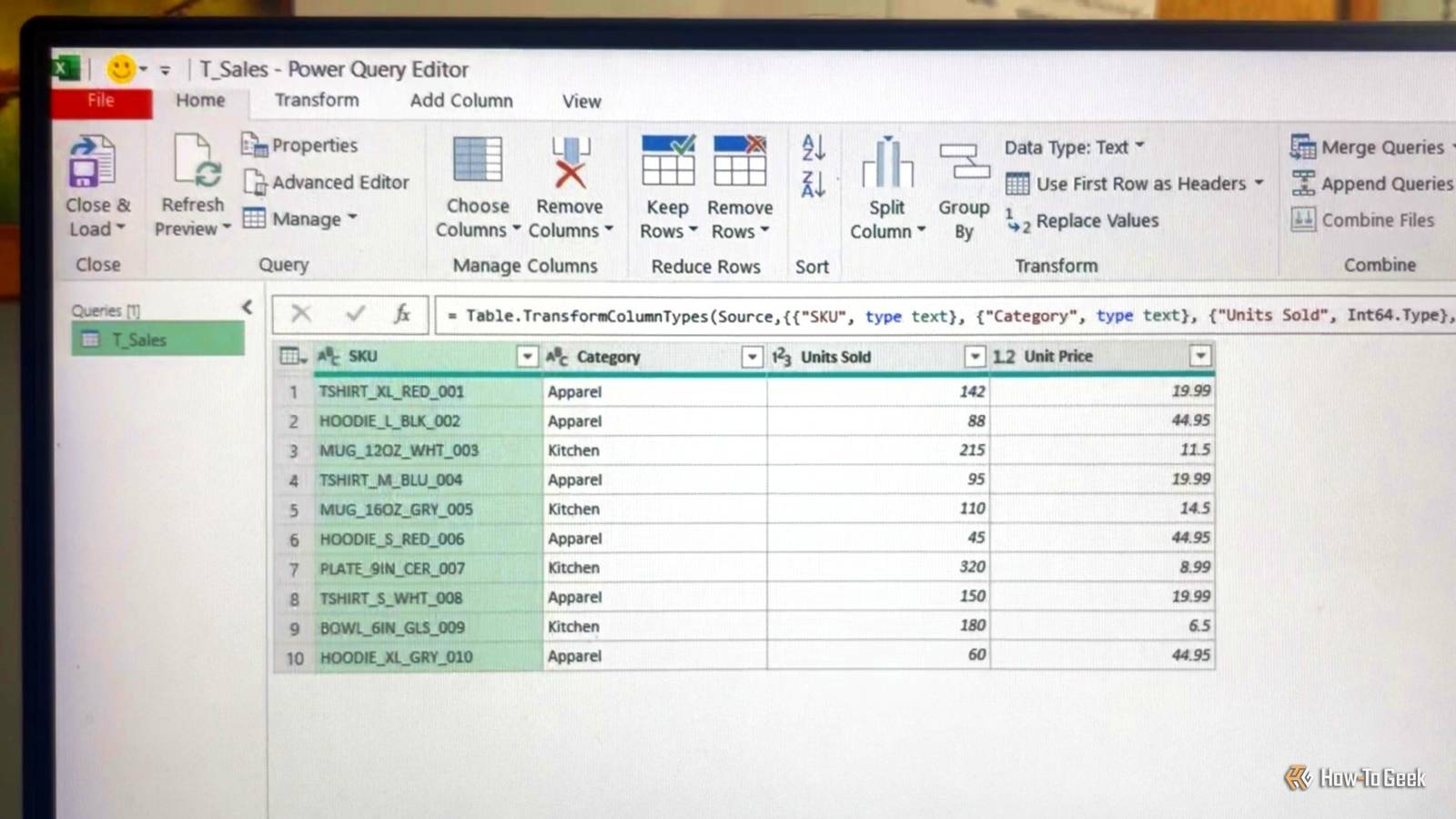
Power Query is one of the most powerful tools in Excel for fixing the dirty data right in front of you. Instead of writing long, nested formulas that are fragile and hard to maintain, you can use the Power Query Editor to record a series of transformation steps. This keeps your cleanup consistent, repeatable, and easy to audit.
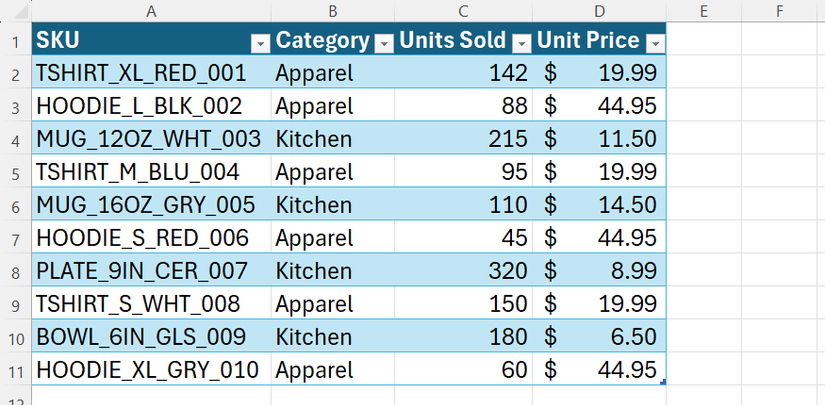
Suppose you’ve been sent this formatted Excel table named T_Sales. It contains a messy SKU column that needs surgical precision, along with a long list of transactions you want to summarize.
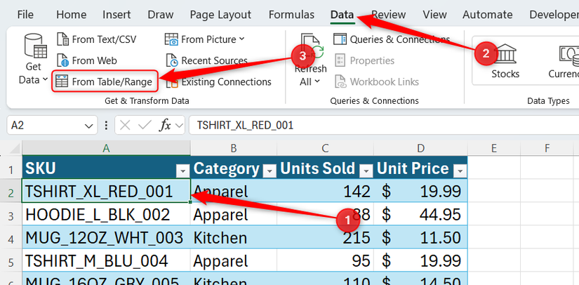
First, load your table into the Power Query Editor. Select any cell within the data, and in the Data tab, click From Table/Range.
Your aim: To take a raw string like TSHIRT_XL_RED_001 and transform it into three separate, clean columns: one for a correctly spelled item name (“T-shirt”), one for the size (“XL”), and one for the color (“Red”).
Extracting an item name or size from a messy SKU usually requires a headache-inducing combination of LEFT, MID, and FIND. In Power Query, however, you can perform a surgical cleanup in seconds.
The first step is to split the SKU column into item, size, color, and ID, and give them clear names:
As you complete these actions, look at the Applied Steps pane on the right. Power Query records every click, one by one, so if you make a mistake, you can simply click the X next to a step to undo it and try again.
Instead of a standard delete, create a “protected list” of columns to keep. This tells Power Query to only ever look for these specific columns going forward. If someone later adds a Notes column to your source data, Power Query will ignore the extra noise, keeping your report lean and schema-proof.
Now that the structure is set, you can fix the formatting of the Item column. This is a two-phase move: the first is a simple transformation that converts block capitals to standard capitalization (for example, “TSHIRT” to “Tshirt”), and the second is to turn “Tshirt” into “T-shirt.”
Finally, you need to turn the three-letter color codes into proper names. You could use the Replace Values tool again, but this would be a time-consuming process that creates several steps. Instead, add a Conditional Column:
Unlike in the standard Excel grid, removing a source column in Power Query won’t break later steps as long as those steps don’t reference it. This is because Power Query processes transformations in a defined sequence. Since you’ve already used Remove Other Columns, a simple Remove here is safe.
Your data is now clean, consistent, and standardized, and you’re ready to move to Workflow 2.
Your aim: To aggregate your transaction list so that instead of seeing every single row, you see a total “Units Sold” value for each category.
Before the final move, you need to branch your data into two independent queries. This preserves the cleaning work you’ve already done as a base layer, allowing you to build the summary on top.
Power Query’s Group By feature lets you perform an aggregation that you might usually reserve for PivotTables. While PivotTables are great for interactive analysis, Power Query is better suited for repeatable, refreshable reporting workflows and avoiding duplicated data structures. Personally, I find the Power Query Editor easier to use than the PivotTable Fields pane.
Now, your data is succinctly summarized into an easy-to-read table.
Finally, click the top half of the split Close & Load button in the Home tab to load your new tables to separate worksheet tabs. If your source data changes, click Data > Refresh All to update both queries.
Using Power Query to automate your workflow is a great way to reclaim your time in Excel. It’s about working smarter by letting the software do the repetitive work for you. Once you’ve mastered these techniques, you’ll find that using Python in Excel is another excellent way to clean and fix data when your datasets get especially complex.
Microsoft 365 includes access to Office apps like Word, Excel, and PowerPoint on up to five devices, 1 TB of OneDrive storage, and more.